
Prelimina 0.3.2 · Updated 2 November 2026
User Guide
Learn Prelimina from your first simulation onwards.
Chapter 1
Getting started
This chapter takes you from nothing to a finished simulation. You will open a bundled sloshing tank, run it, look at the flow, and change one setting. It takes about 15 minutes.
Prelimina is in development. It is useful for exploring ideas, but it is not yet ready for production use. Back up your projects and keep them outside the installation folder.
Choose how to run Prelimina
Prelimina runs as a desktop application or in your browser. The interface is the same in both.
| Browser | Desktop | |
|---|---|---|
| Install | None. Open prelimina.com/app | Windows or Linux installer |
| Graphics | WebGPU in Chrome or Edge 137 or later | Vulkan 1.3 GPU with a recent driver |
| Solvers | FLIP, single phase | FLIP, single phase. FVM, FIRM and the two-phase variants are locked beta features. |
| Results | View only, no results folder | Saved to disk and exported as VTK |
| Examples | One dam break | Four, listed below |
The browser version is the quickest way to see Prelimina. Use the desktop application for your own work. The rest of this chapter follows the desktop application, and the steps are the same in the browser unless a note says otherwise.
In the browser. Firefox and Safari cannot run Prelimina yet. If Chrome reports WebGPU as off or falls back to a software renderer, open
chrome://gpuand check that it shows WebGPU: Hardware accelerated. On a software renderer the simulation stops during initialisation with an error about storage buffers.
Check your computer
| Windows | Linux | |
|---|---|---|
| System | Windows 10 22H2 (64-bit) or newer | 64-bit x86 Linux, glibc 2.28 or newer |
| GPU | From 2015 onwards, Vulkan 1.3, recent driver | The same |
| RAM | 8 GB minimum | The same |
| GPU memory | 4 GB for small scenes, 6–8 GB preferred, 8–12 GB or more for larger work | The same |
| Other | FUSE 2 to mount the AppImage |
These are provisional targets while Prelimina is in development. The Download section always has the current list. macOS is not available yet.
Install the desktop application
Windows
- Download the Windows installer from the Download section.
- Run
Prelimina-0.3.2-win-x64-Setup.exe. The installer is not code-signed yet, so Windows may warn you before it runs. - Start Prelimina.
Linux
- Download the AppImage from the Download section.
- Keep it in a folder you can write to, so that it can update itself.
- Make it executable and start it:
chmod +x Prelimina-0.3.2-linux-x64.AppImage
./Prelimina-0.3.2-linux-x64.AppImage
If your system has no FUSE 2, start it with APPIMAGE_EXTRACT_AND_RUN=1 set in the environment.
Licence. Prelimina is free for noncommercial use. Commercial use, including business evaluation, needs a paid licence before the work begins. See the licence agreement.
Run your first simulation
Prelimina organises work into three stages, shown as tabs at the top of the window:
- Scene holds the physical problem: geometry, fluids, initial state, motion and duration.
- Prepare holds the numerical choices: solver, grid size and time-step controls.
- Simulate runs the solver and shows the results.
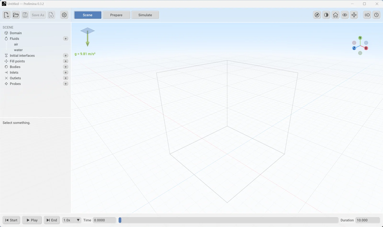
When you start Prelimina it opens an empty, untitled scene in the Scene stage.
Open the example
- Click Open, the folder icon at the top left, or press
Ctrl+O. On a new installation the dialog starts in the examples folder. - Open the
sloshing_tankfolder and choosesloshing_tank.json.
Prelimina copies the example into Documents/Prelimina/Examples and opens the copy. Your edits and results stay there, and the original stays unchanged. Opening the same example again makes a new numbered copy.
Can’t find the examples? Windows may open the dialog in the last folder you used instead. The examples are in the
examplesfolder beside the Prelimina program, by default%LocalAppData%\Prelimina\current\examples.
The tank appears in the viewport. It is 1 m long, 0.6 m high and 0.1 m wide, and closed on all sides. The liquid starts about 0.3 m deep with its surface tilted by 10°. When the simulation starts, gravity pulls that surface flat and the liquid sloshes from side to side.
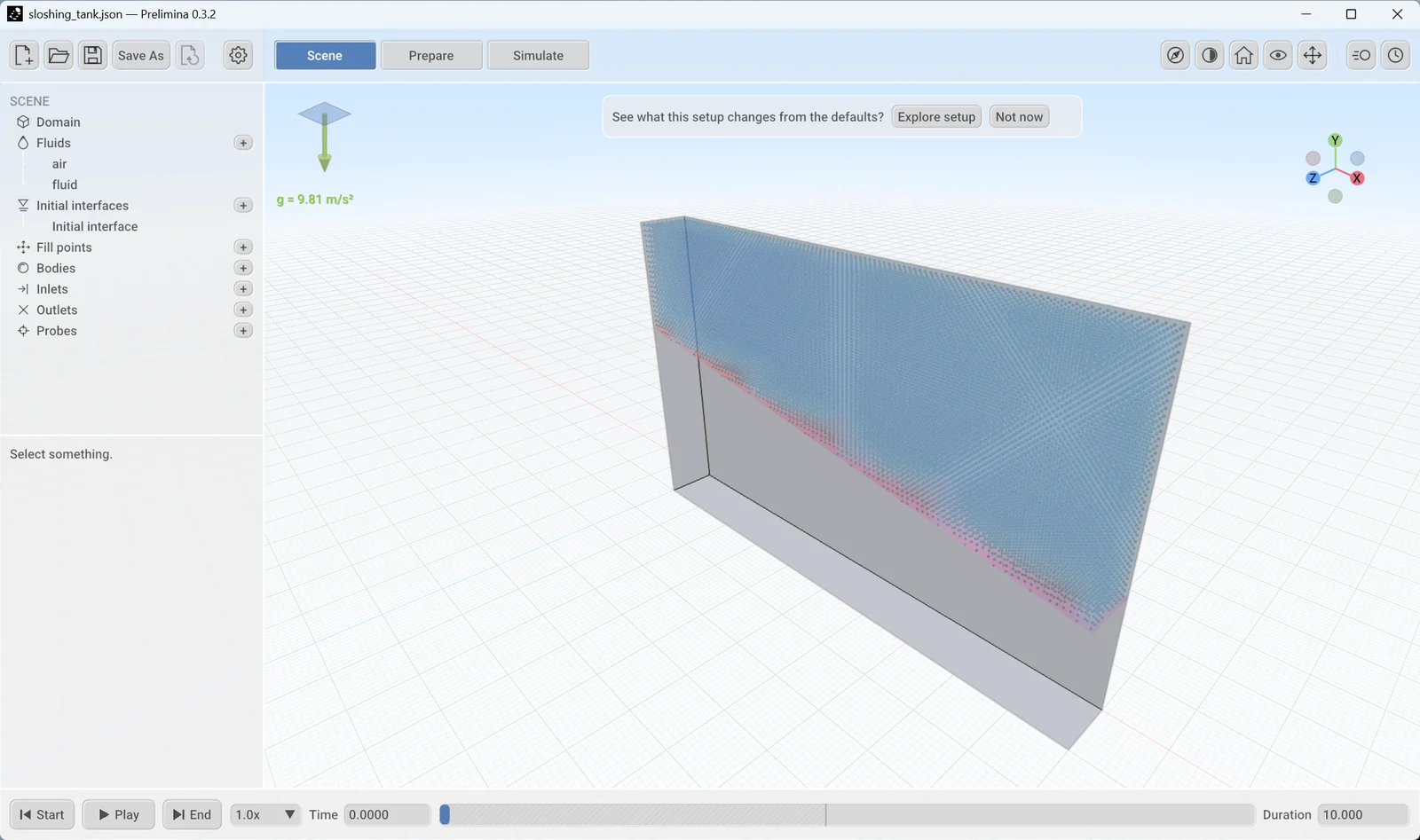
A banner offers to show what this setup changes from the defaults. Click Not now for this first run. You can start the tour later with Explore setup in the settings menu.
Look at the settings
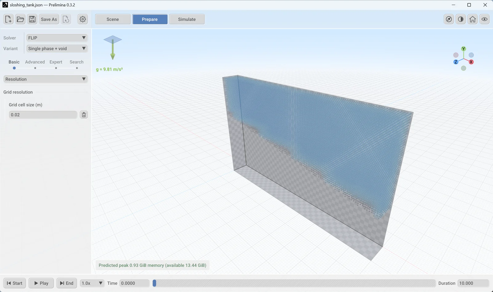
Click Prepare. This example uses the FLIP solver with the Single phase + void variant, which simulates the liquid and treats the space above it as empty. Grid cell size is 0.02 m.
Below the viewport, Prelimina predicts the peak memory for the run and compares it with what your GPU has available. Check this line before you start a large run.
Run it
- Click Simulate. The panel shows Simulation not initialized, because nothing has been sent to the GPU yet.
- Click Run at the bottom left.
The first run on a computer shows Optimizing the simulation for your device. This can take a minute, and later runs start faster. In the browser the first visit can take several minutes.
The liquid then starts to move, and the bar at the bottom shows the simulated time. This example simulates 10 s, which took a little over a minute on an NVIDIA RTX 5080.
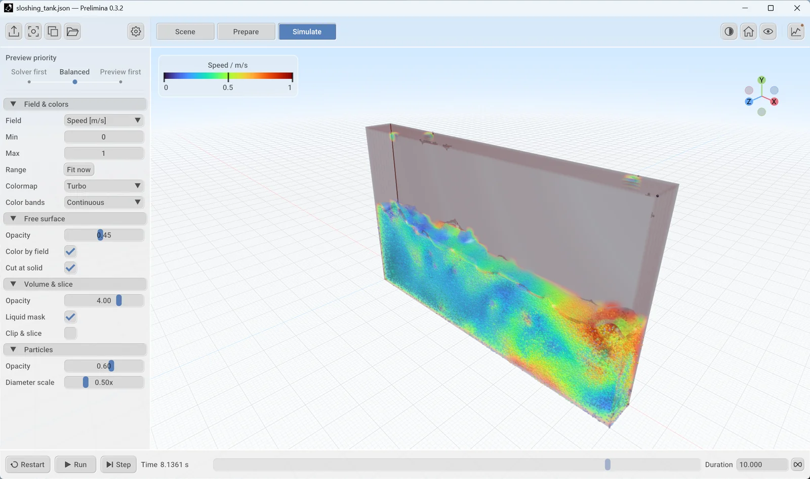
Press Space or click Pause to stop and continue. Step advances one time step while paused. When the bar shows Simulation finished, click Restart to run again from the start.
Look around
These controls work in every stage while the pointer is over the viewport:
| Action | Control |
|---|---|
| Orbit | Left-drag |
| Pan | Right-drag |
| Zoom | Mouse wheel or middle-drag |
| Focus on a point | Double-click it |
| Show everything | Frame all, the house icon at the top right |
| Switch between perspective and parallel view | O |
The small axis gizmo at the top right shows the orientation. Click an axis to look along it.
Read the results
The panel on the left controls what you see. Field selects the quantity. Min and Max set the colour range, and Fit now fits the range to the current values. In this example the speed goes above the default maximum of 1 m/s, so the fastest flow shows as solid dark red until you change the range.
Click the graph icon at the top right to open the live diagnostics. Infos shows the size and speed of the run. Log shows solver messages, and it is the first place to look if something goes wrong.

Find your results
The Output path in Infos shows where this run writes its files. By default this is a results folder beside the setup file.
Four icons at the top left of the Simulate stage handle results:
| Icon | What it does |
|---|---|
| Write results | Pauses and writes the current state as VTK XML, which you can open in ParaView |
| Screenshot | Saves the viewport as a PNG image |
| Copy image | Copies the viewport image to the clipboard |
| Open results folder | Opens the folder in your file manager |
The browser version cannot write results to disk.
Change something and run again
CFD work is a loop of changing a setting and comparing runs. Try it with the grid:
- Click Prepare, set Grid cell size to
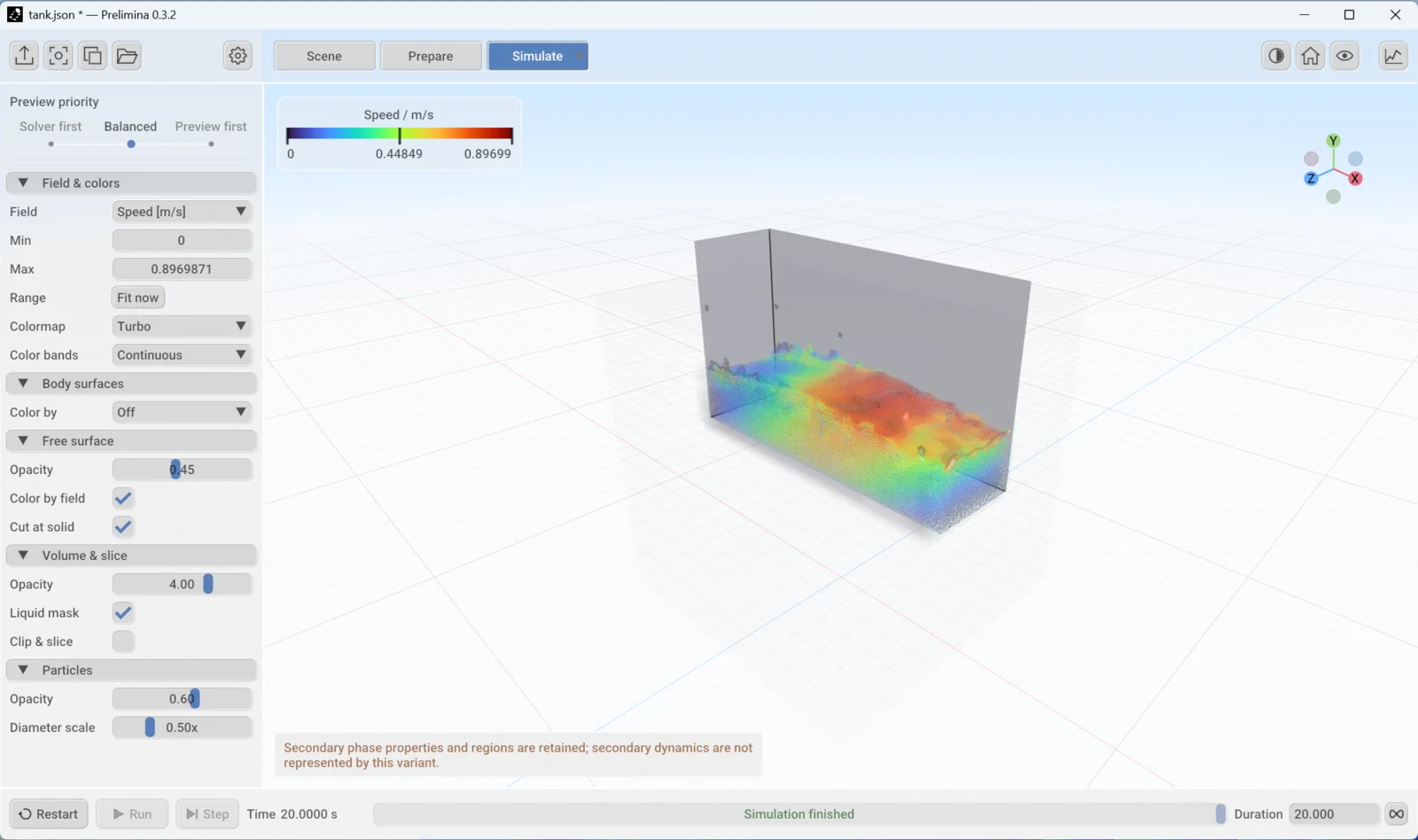
0.01and pressEnter. The predicted memory rises from 0.93 GiB to 1.14 GiB. A*after the file name in the title bar marks unsaved changes. - Click Simulate. Restart has turned amber, which means the simulation on screen still uses the old setting.
- Click Restart, then Run if the simulation is paused.
The new run has 240,018 particles, eight times as many as before, because halving the cell size doubles the cells in each direction. The time step also gets smaller. The 10 s run now takes about three minutes on the same GPU, against a little over one before.
Compare the two runs before you trust either. If the result you care about changes with the grid, the coarser grid was not fine enough.
An amber note may appear about secondary phase properties. It tells you that this variant keeps the air properties in the setup but does not simulate the air.
To keep your change, go back to Scene or Prepare and click Save or press Ctrl+S.
Keep Prelimina up to date
Click the gear icon at the top left and choose Update. A coloured Update available entry appears in the same menu when a new version is out. The same menu has Contact support, which starts an email containing your system details, and About, which shows the version, changelog and licences.
What to try next
- Open the other examples.
drop_in_tankis a small quick case, anddam_break_marinis a 3.22 m dam break with an obstacle.sloshing_kishevreproduces a published experiment at a fine grid, so expect a much longer run. - See how similar cases compare with measurements in Applications.
- See what each feature can do today in Capabilities.
Chapter 2
The workspace
This chapter explains what is on screen and how the parts work together. To follow along, open the sloshing_tank example from Getting started.
The main window
The window has the same layout in every stage: tools along the top, settings on the left, the 3D view in the middle and a time bar along the bottom.
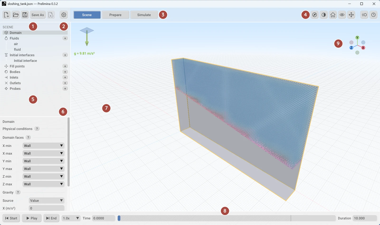
| Area | What it does | |
|---|---|---|
| 1 | File tools | New, Open, Save, Save As and Restore. In Simulate these are replaced by the result tools. |
| 2 | Settings menu | Application settings, updates, support and version details. |
| 3 | Stage tabs | Switch between Scene, Prepare and Simulate. |
| 4 | View tools | Interface theme, camera framing, view options and extra panels. |
| 5 | Scene tree | Everything in the setup, grouped by type. |
| 6 | Properties | Settings for whatever is selected in the tree. |
| 7 | Viewport | The 3D view of the setup or the results. |
| 8 | Time bar | Time, duration and playback controls. |
| 9 | View gizmo | Shows the orientation. Click an axis to look along it. |
The green arrow at the top left of the viewport shows the direction and size of gravity.
The three stages
Each stage changes the left panel and the tools around it.
| Stage | Left panel | Top-left tools | Time bar |
|---|---|---|---|
| Scene | Scene tree and Properties | File tools | Scrubs and plays the preview |
| Prepare | Solver and numerical settings | File tools | Scrubs and plays the preview |
| Simulate | Display settings | Result tools | Runs the simulation |
You can change stage at any time, and doing so never starts, stops or resets a simulation. A run keeps going while you work in Scene or Prepare, and a pulsing green dot on the Simulate tab shows that it is running. A grey dot shows that it has finished.
Changes in Scene and Prepare do not affect a simulation that has already started. They edit the setup, and an amber marker on the Simulate tab and on Restart tells you the running simulation uses an earlier version. Click Restart to apply your changes. The simulation then starts again from t = 0.
Setup files
A setup file is a JSON file that holds everything in Scene and Prepare. It does not hold results. These go in a results folder beside the setup file.
| Tool | Shortcut | What it does |
|---|---|---|
| New | Ctrl+N |
Starts an empty setup |
| Open | Ctrl+O |
Opens a setup file |
| Save | Ctrl+S |
Saves to the current file |
| Save As | Ctrl+Shift+S |
Saves to a new file. Available once the setup has a file. |
| Restore | Goes back to the last applied setup |
A dot on the Save icon and a * in the title bar mean there are unsaved changes. Prelimina asks whether to save them before it replaces the open setup. The Save tools appear only in Scene and Prepare.
Keep meshes and motion files with your setup file. Paths inside a setup are relative to that file, so the folder can be moved as a whole.
There is no undo. Save before a large change. Restore returns to the setup used for the latest simulation start or restart, or to the setup from New or Open if nothing has run yet. It asks first, and it leaves the saved file unchanged. Saving does not move this restore point. In Prepare, a changed setting also has a small revert button beside it.
Select and edit
The Scene tree has one group for each kind of item: Domain, Fluids, Initial interfaces, Fill points, Bodies, Inlets, Outlets and Probes. Click + beside a group to add an item.
Click a row to select it, or click an object in the viewport while in Scene. Properties then shows its settings, and the object is outlined in the viewport. Most sections of Properties have a ? button with a short explanation.
To move a selected object in the viewport, choose a manipulation mode from the toolbar or with a key:
| Key | Mode |
|---|---|
Q |
Select |
W |
Move |
E |
Rotate |
R |
Scale |
Fill points and probes can only be moved. Keys do nothing while you are typing in a field.
View tools
The tools at the top right depend on the stage.
| Tool | Stages | What it does |
|---|---|---|
| Explore setup (compass) | Scene, Prepare | Starts the setup tour |
| Interface theme (half disc) | All | Switches between the light and dark interface |
| Frame (house) | All | Frames the selection, or everything if nothing is selected |
| View options (eye) | All | Opens the list below |
| Manipulation mode | Scene | Selects Select, Move, Rotate or Scale |
| Motion Inspector | Scene | Shows or hides the Motion Inspector panel |
| Timeline Editor | Scene | Shows or hides the Timeline Editor |
| Live diagnostics (graph) | Simulate | Shows or hides the Log, Infos and graph tabs |
A coloured dot on the diagnostics tool means the log has an unread warning or error.
View options controls what the viewport draws. None of these settings changes the physics.
| Option | What it does |
|---|---|
| Filled volume | In Scene and Prepare, previews where the fluid starts: blue for liquid, amber for gas, red for conflicting assignments. This is a coarse preview. |
| Objects | Draws objects hidden, as edges, transparent or opaque |
| Particles, Free surface | In Simulate, shows or hides these layers |
| Sky, Grid | Sets the background. The grid can be hidden, Cartesian or polar. |
| Cut away all objects | Hides the near faces of obstacles as well as containers |
| View gizmo | Shows or hides the gizmo |
| Rotate around picked point | Orbits around the surface under the pointer |
| Rotate horizon with domain | Turns the horizon with a moving domain |
| Orthographic | Uses a parallel view. The O key does the same. |
Boundaries have their own colours: grey for walls, violet for symmetry, green for inlets and red for outlets.
Simulation preview
While you work in Scene and Prepare, Prelimina runs a coarse FLIP simulation of your setup in the background. Grey hatching on the time bar shows how far it has got. Use Play or drag the time bar to watch it.
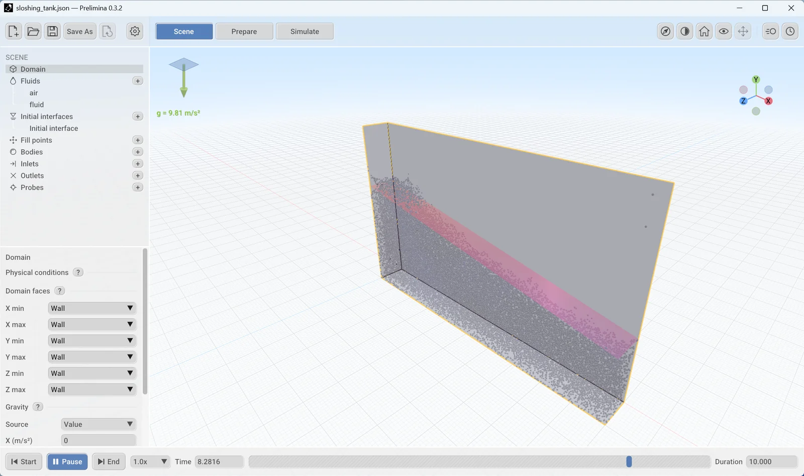
The preview shows quickly whether a setup behaves as you intended, for example whether the liquid starts in the right place or a body moves the right way. It restarts when you change something it depends on. Nothing from it is saved, and Simulate does not use it.
Don’t take numbers from the preview. It always uses FLIP, even if your setup uses another solver, and it runs with its own coarse settings. Thin sheets and splash volume in particular are only indicative. Use Simulate for results.
A simulation and the preview cannot share the GPU. Once a simulation has started, the preview pauses and the time bar offers Release run…. That stops the simulation and frees its memory so the preview can continue. Any results you have not exported are discarded, and the next Run starts from t = 0.
To turn the preview off, clear Compute simulation preview in the settings menu. This is worth doing on a GPU with little memory.
Explore a setup
The tour shows what a setup changes from the solver defaults, which is the quickest way to understand a file from someone else. It takes you through these settings in steps, such as domain and boundaries, then fluids, then solver method. Everything else is dimmed.
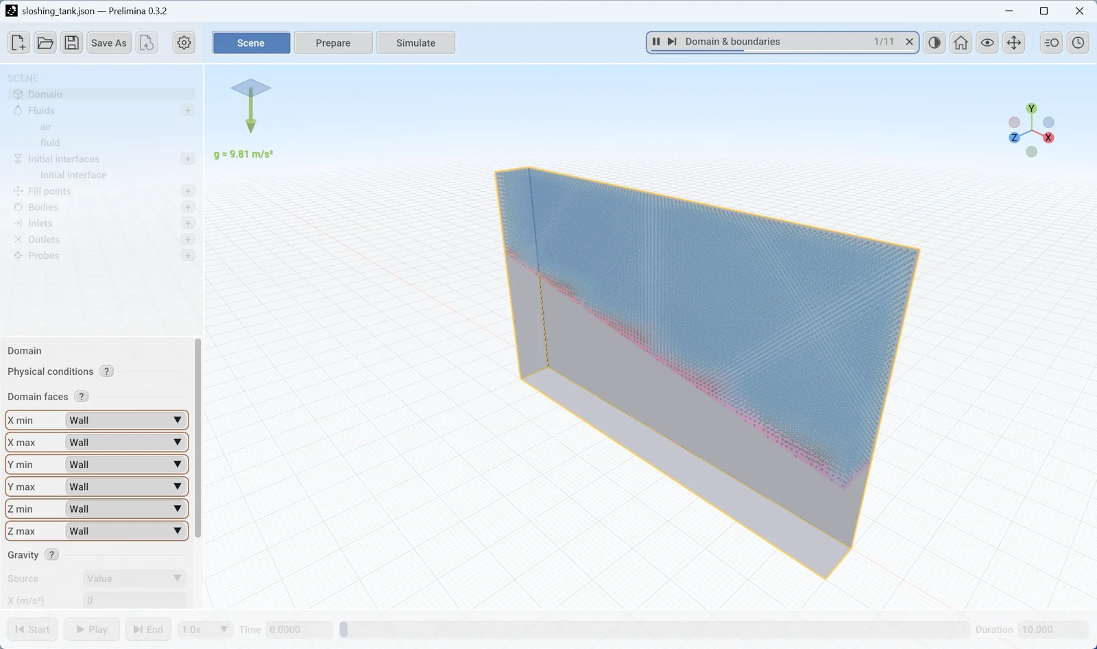
Start the tour in one of three ways:
- Click Explore setup in the banner that appears when you open a file.
- Click the compass icon in the view tools.
- Choose Explore setup in the settings menu.
The tour moves on by itself. Its controls sit in the toolbar: pause or play, next step, the step counter, and a close button. Esc also ends the tour. Hover over the step title to see a table of the changed settings, and over a highlighted row to see its default.
You can keep editing during the tour, and editing pauses it. The tour is available in Scene and Prepare, and going to Simulate ends it.
Settings menu
Click the gear icon to open this menu.
| Item | What it does |
|---|---|
| Compute backend | Shows the compute backend. Released builds use Vulkan. |
| Explore setup | Starts the setup tour, in Scene and Prepare |
| Dark interface | Switches the interface theme |
| Compute simulation preview | Turns the preview on or off |
| Unlock beta features | Enables features that are not ready for general use, including the FVM and FIRM solvers and the two-phase variants. You don’t need it for this guide. |
| Update | Checks for a new version |
| Contact support | Starts an email containing your system details |
| About | Shows the version, system details, changelog and licences |
Keyboard shortcuts
| Keys | Action |
|---|---|
Ctrl+N |
New setup |
Ctrl+O |
Open a setup |
Ctrl+S |
Save |
Ctrl+Shift+S |
Save As |
Space |
Run or pause in Simulate, play or pause the preview in Scene and Prepare |
Home |
Frame the selection, or everything if nothing is selected |
Shift+Home |
Frame everything |
O |
Switch between perspective and parallel view |
Q, W, E, R |
Select, Move, Rotate, Scale, in Scene |
Esc |
Close the tour or cancel the current placement or transform |
When the time bar in Scene or Prepare has focus, the arrow keys step through time, and Home and End jump to the start and end.
Chapter 3
The scene
The Scene stage holds the physical problem. This chapter starts with a complete example that you build yourself, and then explains each part of the Scene tree.
| Item | What it holds | Status |
|---|---|---|
| Domain | Face conditions, gravity and motion of the whole frame | Implemented |
| Fluids | Density, viscosity, surface tension and contact angle | Density and viscosity implemented, the rest experimental |
| Initial interfaces, Fill points | Where the liquid starts | Implemented |
| Bodies | Tanks, obstacles and imported geometry | Implemented |
| Inlets, Outlets | Flow through the boundary | Experimental on domain faces, in development on surfaces |
| Probes | Measurements recorded during the run | Implemented |
Status means the same as on the Capabilities page. Experimental features work, but their interface and defaults may still change.
Prelimina uses SI units throughout: metres, seconds, kilograms and pascals. A new setup has gravity along −Y, so Y is up. You can point gravity in any direction, but this guide keeps the default.
Build a sloshing tank
You will build a tank 1 m long, 0.6 m high and 0.3 m wide, fill it to 0.2 m, shake it from side to side and measure the pressure near one end. This takes about 10 minutes.
Make the tank
- Click New or press
Ctrl+N. - Click + beside Bodies and choose Box. A new box is a 1 m cube centred on the origin.
- In Properties, set Body role to Container, so that the fluid stays inside the box. Set Name to
Tank. - Set Position Y to
0.3. PressEnterafter each value. - Set Scale to
1,0.6and0.3.
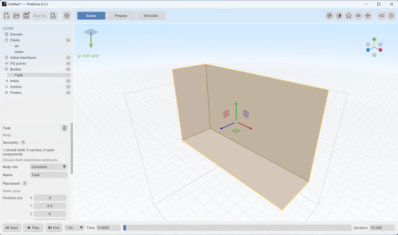
The tank now runs from y = 0 to y = 0.6 m, with its floor on the ground grid. The near walls are cut away so that you can see inside.
Add the liquid
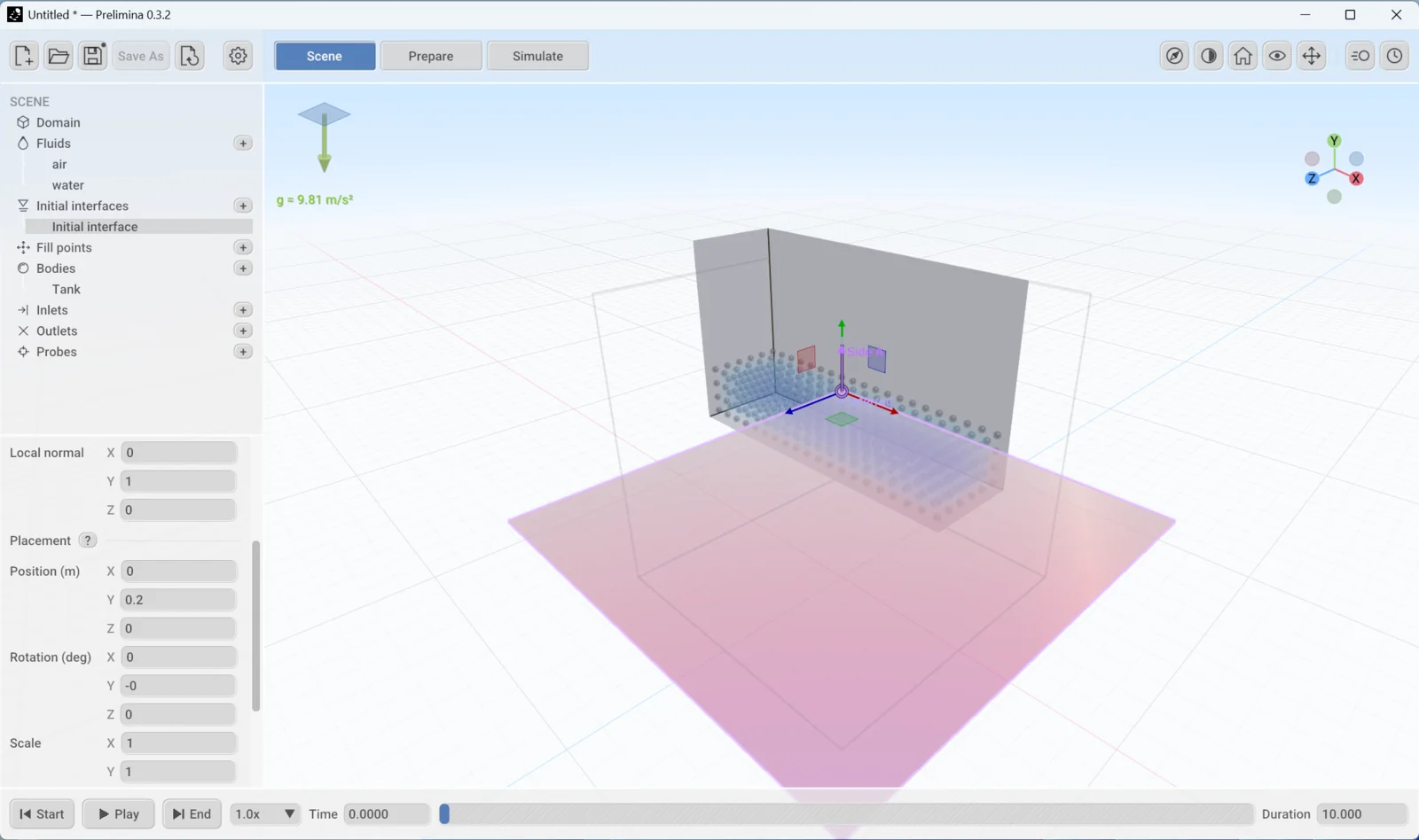
- Click + beside Initial interfaces and choose plane. A plane is the flat surface between liquid and empty space.
- Set Position to
0,0.2and0.
The plane starts at (0.5, 0.5, 0.5), which may be outside your geometry. That is why you move it first. If an error about initial_candidate_unresolved appears, the plane is not yet inside the tank.
Fill volume stays on Automatic, which fills the side of the plane that gravity points to. The liquid appears in blue, and the simulation preview starts in the background. The plane is drawn at a fixed size, but it separates the liquid across the whole tank.
Make it move
- Select Tank in the Scene tree.
- Scroll down in Properties and click Add or edit motion…. The Timeline Editor opens.
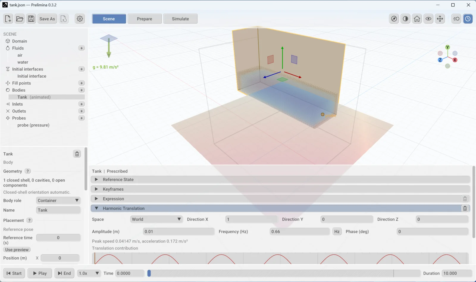
- Expand Harmonic Translation. Its direction is already X.
- Set Amplitude to
0.01and Frequency to0.66.
The tank now moves ±10 mm along X. The panel shows the peak speed, 0.041 m/s, and the tree marks the tank as (animated).
The value 0.66 Hz is close to the lowest natural sloshing frequency of this tank, so the waves should grow. For a tank of length L filled to depth h, that frequency is √(g·k·tanh(k·h)) / 2π, with k = π / L.
Add a probe
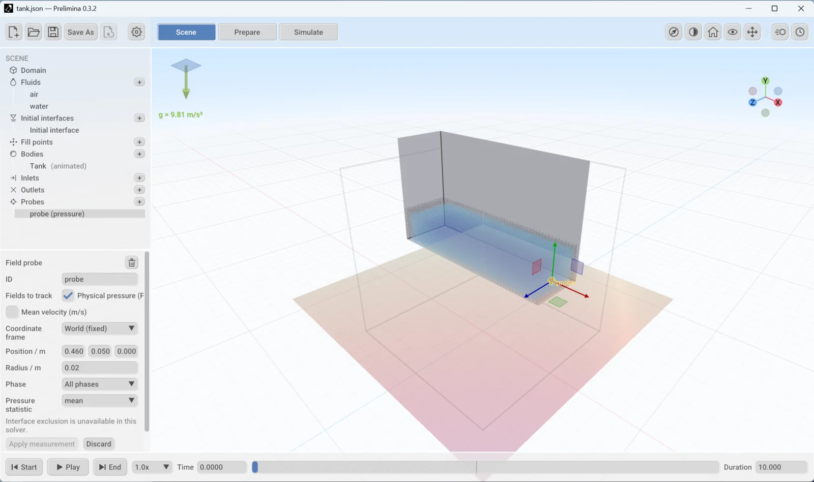
- Click + beside Probes and choose Pressure probe.
- Set Position to
0.46,0.05and0. - Click Apply measurement.
The probe samples a sphere of 0.02 m radius, close to the end wall and 0.05 m above the floor.
Save and run
- Press
Ctrl+Sand save the setup in a new folder of your own. The results will go in aresultsfolder beside it. - Click Prepare and set Grid cell size to
0.02. New setups start at 0.1 m, which is too coarse for this tank. - Click Simulate, then Run.
- Click the graph icon to open the diagnostics, then click Flow. Choose Pressure / probe to follow the measurement.
The run has 60,000 particles. It took under half a minute on an NVIDIA RTX 5080, at about 65 steps per second.
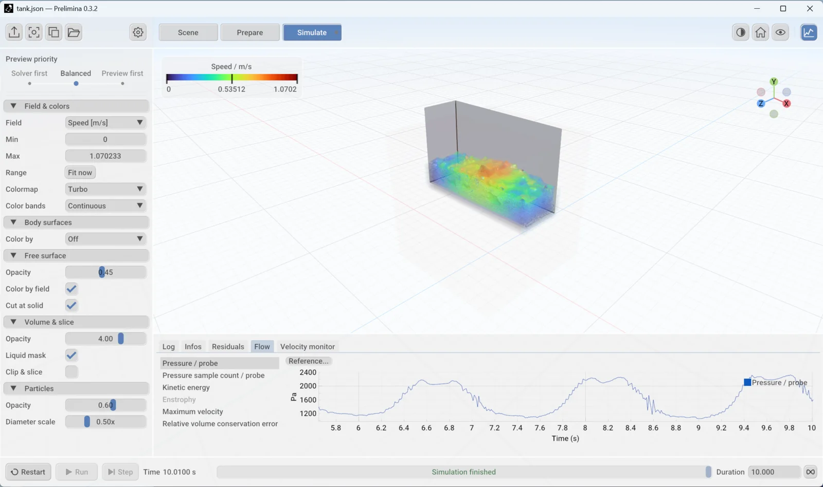
The probe starts near the hydrostatic pressure of 1,470 Pa for 0.15 m of water. It then swings with a period of about 1.5 s, and between 8 and 10 s it ranges from about 1,000 to 2,400 Pa. The waves are still growing when the run ends, so run longer if you need the steady amplitude.
Prelimina writes the probe data to results/probes/measurements.csv without being asked. Each new run starts a new numbered file, so earlier runs are kept.
This is a first run, not a result. A new setup uses a fixed time step of 0.01 s, which is too long for this tank. Even a still tank goes unstable after about 5 s at this step. Prepare a run corrects it and shows how to check a setup.
The domain
The domain is the region the solver works in. How you define it depends on your setup.
Without a fixed size. A new setup has none. The solver sizes its grid from the liquid and the geometry, which is what the tank above uses. The thin grey box in the viewport is a 1 m placeholder and limits nothing. Leave the face settings alone in this kind of setup, because they would attach to that placeholder.
With a fixed size. You need this for domain walls, inlets, outlets and periodic faces. Prelimina 0.3.2 has no field for the domain size, so you add it to the setup file with a text editor. Save and close the setup first, then add lower and upper to the existing domain block:
"domain": {
  "lower": [0, 0, 0],
  "upper": [1, 0.6, 0.3],
  ...
}
Open the file again. The domain box now has that size, and the six faces in Properties apply to it.
Face conditions
Select Domain to set the condition on each face.
| Condition | What it does |
|---|---|
| Wall | Closed face. In FLIP the liquid slips along it freely. |
| Symmetry | Mirror plane. FLIP treats it approximately, as a wall. |
| Periodic | Connects this face to the opposite one |
| Inlet | Flow in through the whole face. See Inlets and outlets. |
| Open (pressure outlet) | Open face at a set pressure. See Inlets and outlets. |
| Solver default | No condition saved. The solver’s default applies. |
A wall face also has Edit prescribed velocity in Timeline…. FLIP saves this velocity but does not apply it, and a warning says so. To move a wall, use a body or reference-frame motion.
Gravity and duration
Gravity has three components in m/s². Each is a number or an expression in time t, or you can choose Keyframed in Source to draw a history. Duration in the time bar sets how long the simulation runs.
Reference-frame motion
Prescribed motion under Domain moves the whole frame, including the grid, and the solver adds the matching inertial forces. It uses the same Timeline Editor as a body. The sloshing_kishev example uses it, with the tank’s acceleration read from a CSV file.
With body motion the tank moves through a fixed grid. With reference-frame motion the tank stays still relative to the grid, which keeps the walls on the same cells throughout the run.
Fluids
A new setup has two fluids, water and air. Click one to edit it, or click + to add a Water or Air preset.
| Setting | Meaning |
|---|---|
| Name | Letters, digits, dots, underscores and hyphens. References update when you rename. |
| Density | kg/m³, must be positive |
| Dynamic viscosity | Pa·s. Zero means inviscid. |
| Rheology | Newtonian, or a non-Newtonian model. Non-Newtonian models are in development. |
Click Fluids itself for the settings shared between them. Primary phase selects the liquid, and Automatic chooses the denser fluid. Surface tension and Contact angle are experimental.
Viscosity needs a solver setting. FLIP ignores the viscosity here unless viscosity is enabled in Prepare, and the Log warns you about this. The default Single phase + void variant also leaves the air out of the simulation, although its properties stay in the setup.
Bodies
Click + beside Bodies to add a Box, Sphere or Cylinder, or choose Mesh file… to import geometry.
Every body has a role:
| Role | Fluid is | Use it for |
|---|---|---|
| Obstacle | Outside the surface | Baffles, hulls, gates and other objects in the flow |
| Container | Inside the surface | Tanks and vessels |
Placement sets the position, the rotation in degrees and the scale. You can also use the Move, Rotate and Scale tools described in The workspace. Scale works around the body’s position, so a box stays centred where you put it.
Import a mesh
Prelimina reads STL, OBJ, PLY, glTF and GLB files, and you do not need a volume mesh.
- Coordinates are read as metres. A mesh in millimetres needs a Scale of 0.001.
- The body keeps the coordinates in the file, so Position starts at 0.
- The view zooms in to the new body. Press
Shift+Hometo see everything again. - Keep the file with your setup. Advanced has Embed compressed fallback, which stores a copy in the setup file.
Geometry in Properties reports what Prelimina found, for example 1 closed shell, 0 cavities, 0 open components. A container should be closed. Prelimina corrects the direction of the faces, but it does not close cracks or weld nearby points, and it rejects non-manifold geometry.
Bodies do not move together
Each body has its own motion, and one body cannot follow another. A baffle inside a moving tank needs the same motion as the tank. With reference-frame motion this problem does not arise, because everything moves with the frame.
Fluid-driven bodies, which the flow moves, are experimental. They have no controls in Scene yet, and this guide does not cover them.
Initial liquid
Two kinds of item define where the liquid starts. Initial interfaces are surfaces that divide the space, and Fill points choose which of the divided regions hold liquid. Neither is a wall: an interface has no effect once the simulation starts.
Initial interfaces
Click + beside Initial interfaces to add a plane, sphere, box or expression, or use Import mesh…. Rotate a plane to start with a tilted surface.
Fill volume chooses which side of the interface fills:
| Fill volume | Fills |
|---|---|
| Automatic | The inside of a closed shape, otherwise the side that gravity points to |
| Along gravity | The side that gravity points to |
| Side A, Side B | The side the arrow points to, or the other side |
| Custom direction | The side a direction you enter points to |
| None | Nothing. The interface only divides the space. |
With no interfaces and no fill points there is no initial liquid.
Fill points
Use fill points when automatic filling cannot work out what you mean, for example with several compartments or nested shapes.
To add one, select an interface and click Add fill point… at the bottom of Properties. Under Suggested position, choose a side. Under Pick on surface, choose a side and click the surface in the viewport. You can also click + beside Fill points.
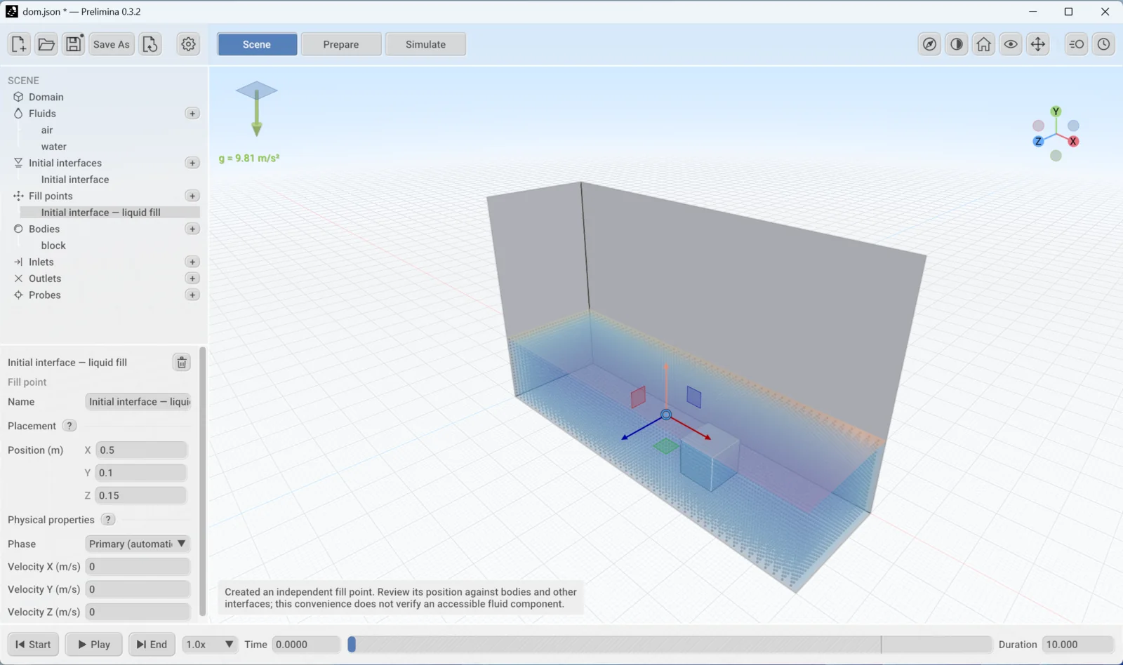
A fill point marks a connected region of space, which then fills completely up to the nearest walls and interfaces.
One fill point replaces all automatic filling. As soon as the scene has a fill point, only regions with fill points fill, so every compartment needs its own. Deleting the last fill point brings automatic filling back. Suggested positions are not checked against your geometry, so look at where the point lands.
Check the fill
Filled volume in View options shows the result in Scene and Prepare: blue for liquid, amber for gas, and red where assignments conflict. It is a coarse preview, so it can differ from the real fill near curved walls and in narrow gaps. The preview particles are a useful second check.
Motion
Select a body or Domain, then open the Timeline Editor with Add or edit motion…, Edit timeline, or the clock icon in the view tools. The Motion Inspector, next to the clock icon, lists the position, velocity and acceleration at the current time.
Reference State holds the starting pose. The motion sources add to it:
| Source | Use it for |
|---|---|
| Keyframes | Hand-drawn histories. Move the time bar, then click Add Key. Translation can use position, velocity or acceleration keys. |
| Expression | A formula in time t for position, rotation, velocity or acceleration |
| Harmonic Translation | Sinusoidal movement, with direction, amplitude, frequency and phase |
| Harmonic Rotation | Sinusoidal rotation about an axis |
| From file | A CSV file with time in the first column |
Space selects world axes or local axes, which rotate with the body. From a file, you can read a full transform, or one of position, rotation, velocity or acceleration. For a full transform, CSV format is t,pos,quat or t,pos,euler.
Click Play in Scene or Prepare, or drag the time bar, to check the motion before you run.
Inlets and outlets
Experimental. Face inlets and outlets need a fixed domain size. Mesh-surface inlets (Rectangle, Circle and Mesh file…) are still in development. Start with short runs and read the Log.
To set up a face, select Domain and choose Inlet or Open (pressure outlet) in the list for that face. It then appears under Inlets or Outlets. You can also use + beside those groups.
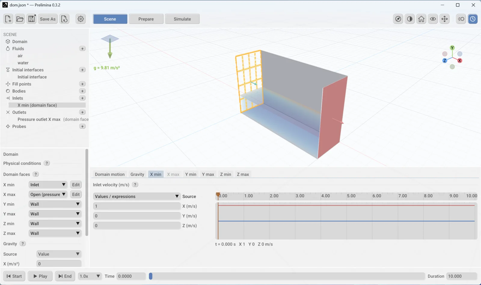
A new inlet flows inward at 1 m/s. Change this in the Timeline Editor, as a number, an expression or keyframes. Inlets need a shorter time step than a new setup uses: at the default 0.01 s, inlet runs stopped with an error within 5 s. Use the settings for inlets and outlets. Adding an inlet can bring back the Optimizing the simulation for your device message for that run.
An outlet has these settings:
| Setting | Meaning |
|---|---|
| Pressure | The pressure on the face, in Pa |
| Pressure type | Static, or Total to include the dynamic pressure |
| Backflow | Clamp reverse flow, or Allow exterior inflow |
| Exterior velocity | Velocity of the flow that comes back in when backflow is allowed |
The pressure is the same over the whole face, so an outlet below a free surface drains the liquid above it.
Probes and measurements
Click + beside Probes to add a measurement. Everything here is recorded to CSV automatically, whether or not the diagnostics are open.
| Item | What it records |
|---|---|
| Pressure probe | Pressure in a small region of fluid |
| Velocity probe | Mean velocity in a small region of fluid |
| Tracer | The path of a point carried by the flow |
| Body measurements | The motion of a body, and optionally the fluid force and moment on it |
A probe can track pressure, velocity or both. Coordinate frame fixes it in the world or attaches it to a body so that it follows the motion. Phase limits it to liquid or gas, and Pressure statistic selects the mean, minimum or maximum.
Set the position in three ways: type it, drag it with the Move tool, or click Pick position in viewport. Click Apply measurement to confirm your changes.
A probe is not a wall sensor. It averages the fluid around a point. To compare with a wall pressure tap, keep the probe in the liquid close to the wall, and check how much the result changes with its position and radius.
Chapter 4
Prepare a run
The Prepare stage holds the numerical choices: how finely the flow is resolved and how the solver advances in time. These settings decide whether a result means anything, and the defaults of a new setup are not always safe. This chapter starts by correcting the tank from The scene, then explains why each change matters.
All measurements here come from Prelimina 0.3.2 on that tank, with FLIP on an NVIDIA RTX 5080. They show how to test your own case. They are not general limits.
Correct the tank
Open the tank you saved in the last chapter and make these changes.
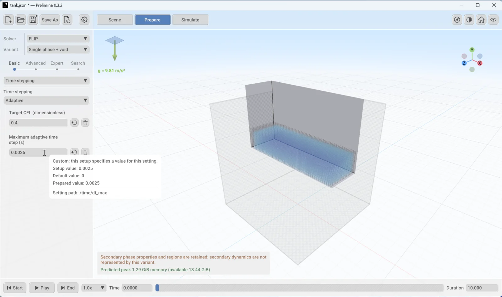
- Click Prepare. Open the list that shows Resolution and choose Time stepping.
- Change the mode from Fixed to Adaptive, type
0.4for Target CFL and pressEnter. - Set Maximum adaptive time step to
0.0025and pressEnter.
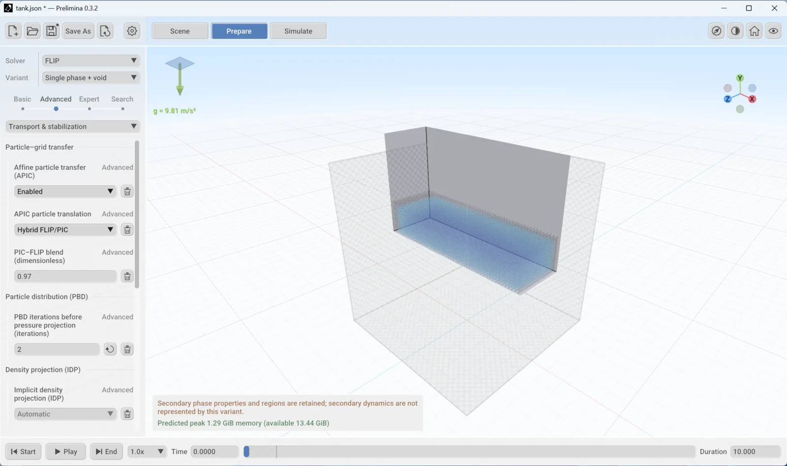
- Move the slider at the top of the panel from Basic to Advanced, then choose Transport & stabilization in the list.
- Set PBD iterations before pressure projection to
2and pressEnter.
- Set Duration in the time bar to
20. - Click Simulate, then Restart if it is available, and Run.
The run takes 8,000 steps instead of 1,000, and 20 simulated seconds took about 100 s. From 12 s to the end, the probe swings between about 900 and 2,400 Pa, with some short spikes above that. Those spikes need care if you are interested in peak pressure.
The rest of this chapter explains these two changes, then shows how to check a setup of your own.
Read the panel
The top of the panel shows Solver and Variant. This guide uses FLIP with Single phase + void, which simulates the liquid and treats the space above it as empty. Other solvers and variants are locked until you choose Unlock beta features in the settings menu, and this guide does not cover them.
The slider sets how much is shown, and the list below it selects a section.
| Level | What it shows |
|---|---|
| Basic | Grid cell size and time stepping only |
| Advanced | The settings you are most likely to change, such as particle capacity and PBD |
| Expert | Everything in the section. Most of it should stay at the default. |
| Search | Finds a setting by name in every section and level |
| Section | What it holds |
|---|---|
| Resolution | Grid cell size and particle sampling |
| Time stepping | Step size and its limits |
| Pressure & convergence | The pressure solver and when it stops |
| Transport & stabilization | How velocities move between particles and grid, PBD and density projection |
| Interfaces & boundaries | Surface reconstruction and solid walls |
| Performance & diagnostics | Particle and grid capacity, extra diagnostics |
| Coupling | Links to external solvers, in Expert only |
Dimmed text in a field means the solver chooses the value. Normal text means your setup specifies it. The bin icon removes your value and returns to the default, and the arrow icon reverts a recent change. Hover over a field to see its Setup value, Default value and Prepared value, which is what the solver will actually use. The Setting path names the same setting in the setup file.
Grid cell size
Grid cell size is the most important setting, and it applies in all three directions. Halving it gives eight times the cells and particles. A new setup starts at 0.1 m, so you will nearly always need to change it.
The grid has to fit the smallest thing you care about, such as the liquid depth, a gap, a baffle or a wave. In the tank, these were the results over the 0.2 m depth with the liquid at rest:
| Cell size | Cells over the depth | Particles | Result |
|---|---|---|---|
| 0.04 m | 5 | 7,500 | Level rose by 18 mm within 2.5 s, at every time step tried |
| 0.02 m | 10 | 60,000 | Level held at the right step size |
| 0.01 m | 20 | 480,000 | Level held at the right step size |
In the moving tank, the finer grid changed the result. The filtered probe swing from 12 to 20 s was about 900 to 2,400 Pa at 0.02 m, and about 500 to 2,900 Pa at 0.01 m, which is 60 % larger. So 0.02 m is enough to learn how this tank behaves, but not to quote a peak pressure. That needs at least one more refinement, and the two results must then agree well enough for your purpose.
The finer run took about 6 minutes against 100 s. It has eight times the particles and, with the step reduced in proportion, twice the steps.
Particles
By default each grid cell starts with 2 particles along each axis, so 8 per cell. This is set under Particle sampling in Resolution at the Advanced level, and you rarely need to change it. Density projection needs an even sampling of 2 or 3 per axis.
Particle capacity is a separate upper limit, under Performance & diagnostics. A new setup allows 1,000,000. If the initial liquid needs more, the run stops at the start and names the setting:
FLIP initialization emits 3840000 particles, exceeding the particle capacity of 1000000 (flip.particles.max_particles)
To estimate the count before you run, divide the liquid volume by the cell volume and multiply by 8.
Time stepping
The time step is the setting most likely to spoil a result without any warning. The Time stepping list has three modes:
| Mode | What it does |
|---|---|
| Default | Lets the solver decide |
| Fixed | Uses the same Fixed time step throughout. New setups use this, with 0.01 s. |
| Adaptive | Changes the step during the run to hold a Target CFL, up to a Maximum adaptive time step |
The CFL number is speed × time step ÷ cell size. It tells you what fraction of a cell the fastest flow crosses in one step. At a target of 0.4, the step shrinks as the flow speeds up.
CFL does nothing in calm liquid. If the flow is slow, the step grows until it reaches the maximum. So Maximum adaptive time step is the limit that protects a resting or slowly moving surface. It shows 0 until you set it, so always enter a value.
How long a step is too long
This test used the tank with no motion, so the correct answer is known: a flat surface and a steady hydrostatic pressure of 1,471.5 Pa at the probe.
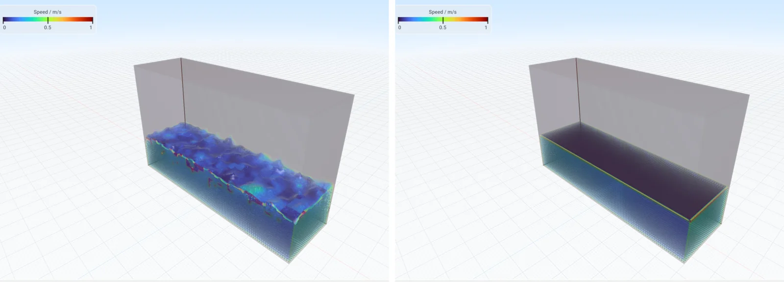
| Cell size | Time step | Over 30 s |
|---|---|---|
| 0.02 m | 0.01 s, 0.005 s | Flat for about 5 s, then rough, with the level about 10 mm too high |
| 0.02 m | 0.0025 s, 0.002 s | Flat throughout, and the probe reads 1,471 Pa |
| 0.01 m | 0.01 s, 0.005 s, 0.0025 s | Flat for about 10 s, then rough, with the level about 5 mm too high |
| 0.01 m | 0.00125 s | Flat throughout, and the probe reads 1,471 Pa |
Adaptive stepping with a target of 0.4 and a maximum of 0.01 s failed in the same way as a fixed 0.01 s, because the liquid never moves fast enough for the CFL limit to act.
The surface stayed flat when the step was no more than one eighth of the cell size, taking metres and seconds. This gives a starting point:
Maximum step in seconds ≈ cell size in metres ÷ 8. That is 0.0025 s for a 0.02 m cell and 0.00125 s for a 0.01 m cell. It comes from these tests on one tank, so check it on your own case.
The instability does not show at first, so a short run can look perfectly clean. Run the check for as long as your real simulation.
A smaller step is not always better
A very small step causes its own trouble. In the moving tank at 0.02 m with no PBD, the liquid at 0.0025 s began to sink after about 15 s. At 0.001 s it had collapsed to half its depth by 20 s, in both of two runs. The step of 0.002 s came through, so this behaviour is erratic and you should not rely on a lucky value. In every collapsed run the simulation still reported success.
PBD iterations prevents this. PBD spreads out particles that have become too crowded, before the pressure step. With 2 iterations, as in the tutorial, the moving tank stayed stable at every step tried, on both grids. These are the 0.02 m results:
| Moving tank, 0.02 m, 20 s | PBD 0 (new setups) | PBD 2 |
|---|---|---|
| Step 0.005 s | Stable | Stable |
| Step 0.0025 s | Sinking after 15 s | Stable |
| Step 0.001 s | Collapsed | Stable |
PBD has a price. In the still tank with 2 iterations, the level stayed within 2 mm at a step of 0.0025 s, but the probe read 1,566 Pa at 0.02 m, which is 6 % high. At 0.01 m it read 4 % high at 0.0025 s, and correctly at 0.00125 s. So allow for an error of this size in mean pressure.
Implicit density projection (IDP), just below it, keeps the liquid at its correct density. It is on Automatic by default, and this is the right choice. With it off, at the default step, the level in the still tank fell by 8 % within 10 s. The Prelimina documentation recommends using it with 2 PBD iterations.
Recommended starting point
| Setting | Closed tank, moving liquid | Inlets and outlets |
|---|---|---|
| Time stepping | Adaptive | Adaptive |
| Target CFL | 0.4 | 0.4 |
| Maximum adaptive time step | Cell size ÷ 8 | Cell size ÷ 8 |
| PBD iterations | 2 | 0 |
| Implicit density projection | Automatic | Automatic |
Inlets are the exception on PBD. With these settings and no PBD, a 1 × 0.6 × 0.3 m channel ran 10 s cleanly at inflows of both 1 m/s and 0.2 m/s, with speeds of 3 to 4 m/s, about what water reaches falling through the channel height. With PBD at 2, speeds jumped to between 8 and 18 m/s. With the default fixed step of 0.01 s, both inflows stopped with this error in the Log, after speeds of 28 m/s:
FLIP density projection candidate validation failed before commit
Turning off density projection stops that error, but the speeds stay at 28 m/s, so the run is still wrong. Reduce the step instead.
Pressure and transport
Leave these at their defaults unless you have a specific reason.
Pressure & convergence controls how accurately each step enforces incompressibility. The solver is PCG, with a limit of 60 iterations. To see how it is doing, open the Residuals tab during a run. Pressure solve residual should sit below its Target line. It stayed below it in the corrected tank.
Transport & stabilization has PIC–FLIP blend, 0.97 by default. A higher value keeps more detail in the flow and a lower value adds numerical damping. Do not use it to tune a result to a measurement.
Check the memory
The line below the viewport predicts the peak GPU memory for the run:
Predicted peak 1.29 GiB memory (available 13.44 GiB)
Available leaves a margin for the driver and other programs, so it is less than the memory on the card. Here it is 13.44 GiB on a 16 GB card. The line is green when there is room, amber when the margin is small or the memory cannot be read, and red when the run will not fit.
The prediction follows the capacity, not your liquid. It is calculated from Particle capacity, plus the grid if the domain has a fixed size. The tank has no fixed domain size, so the line stayed at 1.29 GiB from a 0.02 m cell to a 0.005 m cell, although the finer grid needs 64 times the particles and cannot start at the default capacity. A green line is a check on the capacity you set, not proof that the run will work. Keep Particle capacity close to what you need.
Check a setup before a long run
A run that finishes is not a run that is right. Prelimina reported success for every collapsed tank above. Before you trust a result, work through these checks.
- Rest test. Save a copy of the setup and stop the motion, for example by setting Amplitude to
0. Run it for the full duration. The surface should stay flat, and a probe should read density × gravity × depth. - Compare the level. Look at the liquid at the start and end of the real run. If it has clearly sunk or swollen, stop and change the settings.
- Check the speeds. In the Flow tab, look at Maximum velocity. Estimate a realistic value first. Water falling through a height H reaches about √(2·g·H), which is 3.4 m/s for 0.6 m. Far higher speeds that persist mean a numerical problem, not physics.
- Halve the time step. The result you care about should not change much. Keep PBD on for this, or a small step may fail as described above.
- Halve the cell size and the step together. If the result moves more than you can accept, the coarser grid was not fine enough.
The volume graph cannot see this. Relative volume conservation error in the Flow tab counts particles and multiplies by their fixed volume. It stayed at zero while the liquid collapsed to half its depth. Use the rest test and the level check instead.
For work you will rely on, compare with a measured or analytical case first. Applications shows how this looks.
Chapter 5
Run and read the results
The Simulate stage runs the solver and shows the flow as it develops. This chapter uses the corrected tank from Prepare a run, paused at about 10.6 s.
Decide what you need to keep before you start a long run, because Prelimina saves much less than it shows.
| What | Where it goes | Kept after the run |
|---|---|---|
| The picture in the viewport | Screen only | No, unless you save a screenshot |
| Graphs in the diagnostics | Screen only, about the last second | No |
| Probes | results/probes |
Yes, written during the run for all of it |
| Flow fields at one moment | Write results | Yes, when you click it |
| Flow fields over time | Command line only | Yes |
There is no replay. The time bar in Simulate shows progress, and you cannot drag it back. The flow on screen is the current state of the solver. To look at an earlier moment, restart and pause there, or save fields during the run.
Control the run
| Control | What it does |
|---|---|
| Run, Pause | Starts or pauses the solver. Space does the same. |
| Step | Advances one time step while paused |
| Restart | Starts again from t = 0, using your latest changes |
| Duration | Sets the end time |
| ∞ | Runs with no end time until you pause. Click again to go back to the set duration. |
Preview priority, at the top of the panel, shares the GPU between the solver and the picture. Solver first favours speed, Preview first favours a smooth picture and Balanced sits between them. It does not change the results.
Choose what to show
The panel on the left has one section for each layer of the picture.
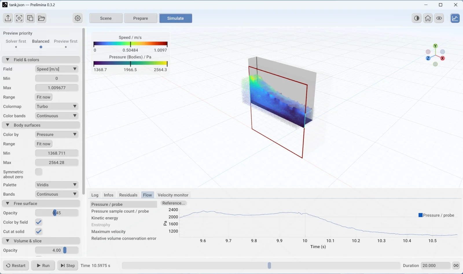
Field selects the quantity:
| Field | What it shows |
|---|---|
| Speed | Flow speed in m/s |
| Grid pressure | Pressure on the grid. See the warning below. |
| Liquid level-set approximation | Distance from the liquid surface, in metres, negative inside the liquid |
| Grid density | Density on the grid, in kg/m³ |
| Curvature | Curvature of the liquid surface, in 1/m |
Min and Max set the colour range. Fit now fits it to the current values. To compare two moments or two runs, type the same range for both, otherwise the same colour means different values. Colormap and Color bands change the colours, and bands make levels easier to read.
Don’t read pressure from the Grid pressure colours. In 0.3.2 the viewport shows this field too high by a large factor. In the tank at a 0.02 m cell size, it showed −16,462 to 128,224 Pa, while the exported field for the same moment ran from −329 to 2,564 Pa, a factor of exactly 50. The shape of the field is still useful. For values, use a probe, Body surfaces or exported results.
Body surfaces colours a body by the pressure of the fluid next to it. Choose Pressure in Color by. It has its own range controls, and areas with no fluid beside them stay grey. Wall shear stress was greyed out for the tank, which does not simulate viscosity.
| Section | Use it for |
|---|---|
| Free surface | Opacity of the liquid surface, and whether the field colours it. Cut at solid trims the surface at walls. |
| Volume & slice | Opacity of the field inside the liquid. Liquid mask limits it to the liquid. |
| Particles | Opacity and size of the particles |
Move any Opacity slider to zero to hide that layer.
Look inside with a slice
- Open Volume & slice and select Clip & slice. A coloured plane appears, and everything on one side of it is hidden.
- Choose X, Y, Z or Arbitrary in Plane. Arbitrary adds a Plane normal.
- Drag Plane position, from 0 to 1 across the flow.
- Set Contours to draw lines of equal value on the slice.
Select Plane handle to move or rotate the plane in the viewport. The hidden side follows the camera, so orbit around to see the other side.
Read the diagnostics
Click the graph icon at the top right to open these tabs. A coloured dot on the icon means the Log has a new warning or error.
| Tab | What it shows |
|---|---|
| Log | Solver messages, with a filter, a level list and Copy |
| Infos | Time, time step, size, speed and the output path |
| Residuals | How well each step was solved, against its target |
| Flow | Probe readings, kinetic energy and maximum velocity |
| Velocity monitor | Maximum and mean speed, and the count of invalid particles |
The graphs in Residuals and Flow cover about the last second of the run, so they suit checking the flow as it runs, not reading a history. For a full record, use the probe file below.
Velocity monitor only checks whether the speeds are finite numbers. As it says on screen, it does not show that the solution is sound. Prepare a run has the checks that do, and explains why Relative volume conservation error can stay at zero when the volume is wrong.
Compare with a measurement
You can draw a measured curve over any graph in Flow or Residuals.
- Select the graph, then click Reference… and choose a CSV file.
- Give the file a header row. It needs a time column and a value column, with the values in the units shown on the graph.
- Click Align if the curve needs adjusting.

| Align setting | What it does |
|---|---|
| Time column, Value column | Selects the columns to use |
| Time scale | Seconds per unit of the time column, for example the period T for data in t/T |
| Time offset | Shifts the curve in time, to line up the phases |
| Repeat every | Repeats the curve with this period. 0 shows it once. |
| Value scale | Multiplies the values |
This is a quick visual check, and it only covers the last second of the run. For a real comparison, use the probe file and your own plotting tools. Note any offset you apply, because it is part of your result.
Save the numbers
Probes
Every probe writes to results/probes during the run, with no action from you. The first run writes measurements.csv, and later runs write measurements-2.csv and so on. A paused or stopped run keeps what it has written so far.
The file has one row per step for each series, so filter it by series_id. The tank probe has two series, the pressure and the number of particles it sampled.
| Column | Meaning |
|---|---|
frame, time_s, dt_s |
Step number, time and time step |
series_id |
Which measurement, for example pressure_probe.probe.pressure_pa |
value, units |
The reading and its units |
availability |
available when the value is valid |
sample_count |
Particles behind this reading |
x_m, y_m, z_m |
Where the probe was |
This Python script reads one series and prints its mean:
import csv

rows = [r for r in csv.DictReader(open("measurements.csv"))
        if r["series_id"] == "pressure_probe.probe.pressure_pa"
        and r["availability"] == "available"]
t = [float(r["time_s"]) for r in rows]
p = [float(r["value"]) for r in rows]
print(len(p), "samples, mean", sum(p) / len(p), "Pa")
The first sample of a run can be 0, because the probe has no pressure before the first step. Leave it out of averages.
Fields at one moment
Write results, the first icon at the top left, saves the current state.
- Click Write results. The run pauses.
- Check the Folder, which is the
resultsfolder by default. - Click Write now, then Close.
Each click adds a step_NNNNNN folder and an entry in results.vtm.series. One frame of the tank took about 10 MB:
| File | What it holds |
|---|---|
particles.vtp |
Particle positions and velocities |
free_surface.vtp |
The liquid surface as a mesh |
grid/*.vti |
Grid fields, including pressure and velocity |
results.vtm.series |
The list of saved moments. Open this one. |
A folder can only take later moments of the same run. After a Restart, choose a new folder.
Fields over time
The application saves fields only when you click. Record results, which saves them at regular intervals, is a locked beta feature in 0.3.2. To record a series without unlocking it, use prelimina_cli, which is beside the Prelimina program:
prelimina_cli tank.json --backend vulkan --output metrics.csv --vtk-dir fields --vtk-every-time 0.5 --vtk-product volume --vtk-field pressure --vtk-field velocity
This writes the grid fields every 0.5 s of simulated time, and --duration overrides the end time. Each run records one product, and FLIP has volume, particles and free_surface. Without --vtk-product you get particles and the free surface. Run the same setup again for another product.
The command line has no results/probes folder. Probe values are in metrics.csv instead, as result_pressure_probe_... columns, with ; as the separator and several hundred columns in all.
Start small. The tank with particles and surface took about 1.4 MB per frame, and a fine grid or a short interval can fill a disk quickly.
Pictures
Use Screenshot to save the viewport as a PNG, and Copy image to put it on the clipboard. Neither includes the panels. The folder icon opens the results folder.
Open results in ParaView
- In ParaView, choose File > Open and select
results.vtm.series. - Click Apply. The time controls step through the saved moments.
- Use the block list to choose particles, grid or free surface.
| Use this | Not this |
|---|---|
Grid pressure, in Pa |
Particle pressure, which is 0 in every particle in 0.3.2 |
Grid velocity, where velocity_valid is 1 |
Grid values outside the liquid |
Exported grid pressure is in Pa, and its maximum matched Body surfaces at the same moment, so ParaView is the place to measure a field.
If a run stops
The bar shows Initialization failed or the run stops, and a message appears in the viewport and in the Log. Copy it with Copy if you need to contact support.
| Message contains | Cause | What to do |
|---|---|---|
exceeding the particle capacity |
The initial liquid needs more particles than allowed | Raise Particle capacity. See Particles. |
density projection candidate validation failed |
Usually a time step that is too long | Use the recommended settings |
A run that finishes can still be wrong, so a clean Log is not enough. See Check a setup before a long run.